[Deep Dive: NetsPresso®] From Quantization to Graph Optimization: A Step-by-Step Model Deployment Pipeline

Jaehoon Lee
Technical Content Manager, Nota AI
Series Notice: NetsPresso® Technical Blog, Part 2
In Part 1, we walked through a scenario of deploying Llama 3.2 1B on an edge device to illustrate the NetsPresso® workflow. The flow covered building an optimization pipeline with four CLI commands from np workspace init to np run, automatically exploring multiple configurations with sweep, and comparing pre- and post-optimization results through Probe.
In this Part 2, we step inside the three stages that np run executes under the hood: --steps aq, go, gq. You can follow along without having read Part 1, since we will unpack the necessary context at each stage. If you are curious about Part 1, you can read it here.
Three Bottlenecks in Target Device Deployment
The number of operators defined by PyTorch continues to grow each year. The range of computations a model can express has expanded along with it. The pace at which hardware SDKs on target devices support these operators, however, has not kept up. It is common to finish training a model only to find that the chip cannot execute the required operators.
Even when a model can be loaded onto the device, the work is not over. To fit within constrained memory and compute, the model must be trimmed down. Recent techniques such as AWQ have made it much easier to reduce weights to INT4. The difficulty lies in applying these algorithms to your own model and device without accuracy loss.
The biggest issue is that this entire process is disconnected. Outside of a handful of large vendor environments with fully integrated software stacks, quantization, graph optimization, and compilation tools remain fragmented across countless embedded devices and chipset environments. Input and output formats must be converted step by step, and switching target devices often means reviewing the whole pipeline from scratch.
NetsPresso® three-stage optimization engine (AQ, GO, GQ) was built to resolve these fragmented bottlenecks within a single pipeline.
Advanced Quantizer (AQ): Seven Quantization Algorithms in One Pipeline
Four Barriers That Individual Libraries Leave Unresolved
AQ provides seven core algorithms that have become the standard for PyTorch-level quantization, all at the first stage of the pipeline. The coverage includes ultra-light weight compression methods (AWQ, GPTQ, AutoRound, HQQ), methods that handle activation outliers (QuaRot, SmoothQuant), and basic round-to-nearest (RTN) for sanity checks. We continue to integrate newly emerging quantization methods into the pipeline and are rapidly expanding the supported pool.
These algorithms can, of course, be used directly through open-source libraries or paper implementations. Applying multiple algorithms to a single model for comparison, however, is cumbersome. Passing the optimization result cleanly into the next stage is also difficult. Understanding the algorithms in theory is separate from working with them in practice, where engineers have to resolve the following four barriers on their own.
Environment conflicts across libraries: Major algorithms such as AWQ, GPTQ, AutoRound, and HQQ are scattered across different packages. The torch and CUDA versions they require also differ. Testing multiple algorithms in a single environment is itself a significant hurdle.
Research-grade code limitations: Most recent open-source quantization implementations are tied to specific architectures or data types. Cross-experimenting by switching targets or datasets is difficult, which makes consistent performance comparisons across algorithms hard to produce.
Fragmented data preprocessing formats: Each library expects different data shapes and sequence lengths. Even when using the same data, preprocessing has to be repeated as many times as there are algorithms.
Disconnected output formats: Most algorithms support only a limited set of output formats. To pass quantization results to downstream stages such as target-device compilation, framework-specific conversion adapters have to be prepared separately.
AQ unifies these complex dependencies and formats into a single YAML configuration. Calibration data is loaded automatically from the HuggingFace Hub, so there is no need to rewrite preprocessing code for each library. The sweep feature introduced in Part 1 also lets you compare all algorithms on the same evaluation metric in a single run. The value of AQ therefore lies not in merely listing algorithms, but in making fragmented techniques usable inside one pipeline.
Why AQ Is the First Stage of the Pipeline
Algorithms such as AWQ and GPTQ operate directly on the original PyTorch weights. Once the model is converted into a graph representation, the sensitive weights at the core of the model can no longer be safely protected. Missing this timing causes issues in later stages. When the model's computational structure is later changed or data precision is substantially reduced, accuracy tends to shift significantly. In the end, the quantization settings have to be redone from the beginning.
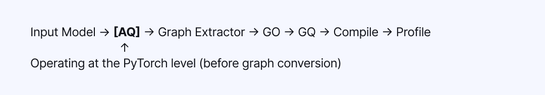
Table 1: Position of AQ in the NetsPresso® optimization pipeline (operating at the PyTorch level, before graph conversion)
There is another reason NetsPresso® places AQ at the first stage: it automatically normalizes fragmented quantization results into NetsPresso® common intermediate representation (NPIR). A model that passes through AQ continues without interruption through GO, GQ, compilation, and profiling. Even when the quantization algorithm is swapped mid-pipeline, the downstream stages do not need to be rebuilt.
NPIR and Graph Optimizer (GO): Device-Specific Graph Optimization
NPIR: A Common Intermediate Representation Built for Optimization
After AQ processing, the PyTorch model is converted into a new graph form for the next stage. This is NetsPresso® proprietary intermediate representation (NPIR). The subsequent GO and GQ stages all operate on top of NPIR.
The following sections examine the specific structure of NPIR that connects GO and GQ without breaks, first reviewing its characteristics and then showing how GO reassembles a model differently for each device.
ONNX vs NPIR: General-Purpose Exchange Format vs Optimization-Focused Representation
When an intermediate representation is needed for model conversion, ONNX is the common choice. Major deep learning frameworks (PyTorch, TensorFlow) and inference engines (TensorRT, OpenVINO) mostly support it. The main reason for its adoption is universality: "once converted to ONNX, it can run anywhere."
NetsPresso® nonetheless built its own NPIR for two clear reasons. The first is to overcome the limits of representation. The second is to deliver optimization and compression that fit fragmented devices in a single, coherent flow.
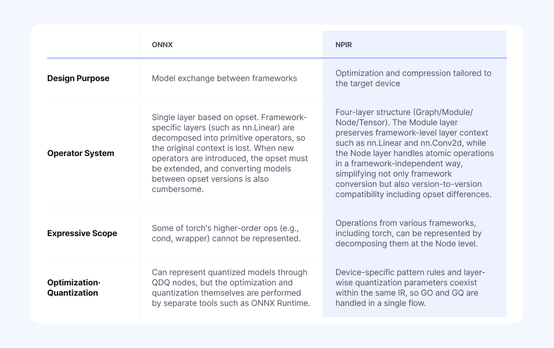
Table 2: Comparison of ONNX and NPIR in terms of design purpose, operator system, expressive scope, and optimization approach
This structural difference surfaces immediately in practice. In an ONNX-based workflow, framework-specific layer information is lost. For example, PyTorch's nn.Linear is decomposed during ONNX conversion into a MatMul operation (plus Add when bias is present). As weights and bias are scattered across separate atomic operators, the fact that they once formed a single linear transformation layer disappears.
Since layer-level decisions, such as which quantization scheme to apply to an entire Linear or whether to group a specific combination like Conv + BatchNorm as a single unit for conversion, all require knowing "what layer this originally was," this loss of information becomes a significant problem. Once the fact that split operators used to form one block is lost, graph conversion, optimization, and quantization have to be stitched together with different tools.
NetsPresso® NPIR is different. It preserves the context of the original layer at the Module level while handling the smallest atomic computations (Nodes) individually. As a result, operator patterns grouped during an earlier optimization stage carry over as computational units for the next quantization stage without any break. Because complex operators are also split into Nodes, NPIR is relatively free from the conversion compatibility issues that surface every time the ONNX opset changes. When the target device changes, the pipeline does not have to be reassembled from the beginning.
Graph Optimizer: Device-Specific Optimization Based on 150+ PatternsOne Configuration Is Not Enough: Compare Multiple Settings at Once
Reducing a model's size through quantization does not automatically make it fast on the target device. In practice, engineers hit three main barriers at this stage.
Unsupported operators that block execution: Cases where the device SDK does not support a specific operator, so the operator cannot run on the neural processing unit (NPU). An example is LayerNorm being rejected on the Ethos-U NPU.
Performance degradation from inefficient compute paths: Cases where the operator is supported, but execution falls onto a significantly slower path. For example, Einsum may be supported, but converting it to MatMul can be several times faster.
Fragmented optimal answers across hardware and backends: The fixes for the above two issues vary by device and backend. An operator that should be left alone on XNNPACK may need to be split on Ethos-U, and vice versa, so a rule validated in one place cannot simply be reused in another.
NetsPresso® GO first strips out inefficient operations through graph transformations that preserve mathematical equivalence. Let us look at one example of how a transformation actually happens.
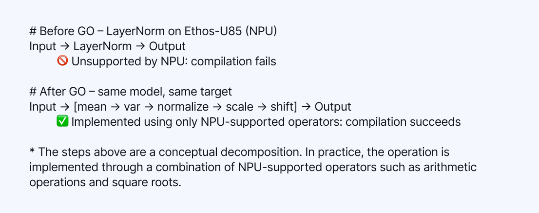
Table 3: Example of how GO operates, decomposing LayerNorm into a combination of NPU-supported operators on Ethos-U85
In the example above, GO rewrites a LayerNorm that Ethos-U85 cannot handle into a combination of NPU-supported operators only, resolving the compilation failure. Conversely, on a backend that has a dedicated LayerNorm kernel, decomposing LayerNorm would actually be slower, so GO keeps LayerNorm intact.
In this way, GO applies target-aware pattern matching and produces graphs with entirely different structures for the same model depending on the device. NetsPresso® maintains a pool of more than 150 optimization patterns, and dynamically selects only the rules most beneficial for the given target, whether NPU or CPU.
These rules are not merely theoretical optimizations. They are field data accumulated as Nota AI carried out numerous commercial projects, directly addressing hardware environments that range from ultra-small chips (Arm Cortex-M) to NPUs and server-class LPUs.
Splitting unsupported operators, replacing slow operators with faster ones, setting the boundaries of quantization blocks, and re-validating everything whenever the device changes: the number of variables to consider at this stage is endless. For any individual team, validating this vast process from scratch would require enormous cost and time. NetsPresso® GO addresses this region with patterns proven in real deployments.
Graph Quantizer (GQ): Automatic Layer-Wise Mixed-Precision Assignment
Capability Map and Fail-Fast: From Scheme Validation to Calibration
The graph optimized by the GO engine is passed to the GQ engine, entering the final compression stage. If AQ was the process that protected weights from damage, GQ is the engine that converts the floating-point (FP32/FP16) weights and activations into integer formats (INT8/INT4) and fixes the final model size and inference speed.
GQ, however, does not apply this conversion uniformly across the entire graph. Because different devices support different data types for different operators, it traverses the graph and applies a quantization scheme that matches the kernel supported for each operator. This stage aligns the quantization scheme selected by the user with the range actually supported by the target hardware.
A quantization scheme must be determined by the physical constraints of the target hardware. NetsPresso® embeds the support specifications of major devices as a "Capability Map" to control this process systematically.
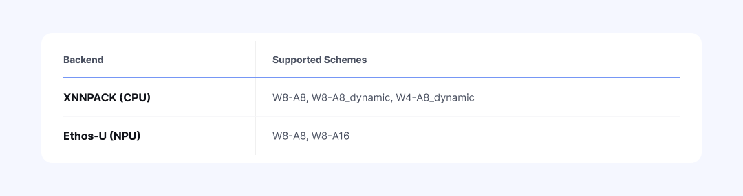
Table 4: Quantization schemes supported by each backend
As shown in the table above, the CPU (XNNPACK) supports dynamic quantization that requires real-time scale computation, while a specific NPU (Ethos-U) allows only static quantization schemes. If a scheme outside the device's constraints is configured (for example, W4-A8_dynamic on Ethos-U), the pre-validator triggers a fail-fast mechanism before quantization begins. Engineers can thereby avoid compilation failures from incorrect settings and unnecessary runtime wait times.
Once scheme validation passes, calibration begins. GQ directly feeds the model with data representative of the user's production environment and measures the activation range for each layer (computing scale and zero-point values). On top of that, GQ provides multiple calibration methods suited to different data distributions, such as MinMax, percentile, and histogram, so that accuracy drops are minimized even in models with outliers.
Automatic Mixed Precision (AMP): Automatic Search of Layer-Wise Quantization Sensitivity
Uniform quantization, which applies the same bit width to every layer, is simple. It is not always optimal, however, because different layers respond to quantization with different sensitivities. For a model like Llama 3.2 1B, where quantization modules number around one hundred, the combinatorial space reaches roughly 2^100. Exhaustive manual search is effectively impossible.
NetsPresso® AMPsolves this problem with an automatic search algorithm. After measuring the quantization sensitivity of each layer, AMP assigns higher precision to sensitive modules and lower precision to the rest. The table below, for example, shows the result of assigning FP32 to sensitive layers and INT8 to the remaining layers.
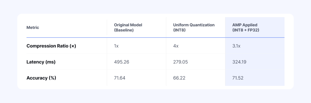
Table 5: Performance comparison of the vit_b_16 model across original, uniform quantization (INT8), and AMP (FP32+INT8)
AMP shows its value when uniform quantization has already caused accuracy to drop. It keeps the overall model size small while raising precision only on sensitive layers, suppressing the accuracy loss. It shortens the painful task of manually testing hundreds of combinations into a single run.
To further refine the results generated by AMP, Manual Mixed Precision mode lets you adjust specific layers directly. This is a practical workflow that uses AMP's automatic assignment as a baseline and edits only the parts that need attention. If you want to control detailed candidate precisions or search ratios, you can specify them directly in the configuration file (run.detail.yaml).
Compiler and Profiler: From Cross-Compilation to On-Device Benchmarking
After AQ, GO, and GQ, it is time to convert the optimized NPIR graph into binary code that the actual device can read.
The Compiler module takes this optimized graph and generates a binary for the target environment (for example, an ExecuTorch-based .pte file). Whether the target is a CPU (M4) or an NPU (Ethos-U85), engineers do not have to manually set up a complex cross-compile environment. The optimal conversion path is determined automatically based on the project configuration.
Once converted, the binary moves directly to the target board and meets the Profiler. The Profiler measures latency and memory usage on the device. It then presents the results in a clean tabular form through the np report command. You can see directly how much lighter the original model has become across the three stages.
If a target board is not immediately available, you can leave the profiling section of the configuration file (run.yaml) empty and run only the optimization pipeline first.
In effect, the Compiler and Profiler make the optimized model immediately executable on the target device and cross-verify its performance. They form the final step that completes the NetsPresso® pipeline end-to-end.
Optimization Benchmark: Llama 3.2 1B Measured Results
Llama 3.2 1B Quantization Benchmark: Full AQ + GO + GQ Pipeline
Let us revisit the final result that we saw through np report in Part 1. This time, we analyze, from a technical perspective, exactly how each stage of the optimization pipeline (AQ, GO, GQ) transforms the model.
[Stage 1] AQ: 87% Memory Reduction
This is the direct outcome of reducing weights to 4-bit (INT4). At this point, latency does not change. AQ only changes how weights are stored as a first pass; the execution graph that performs the computation has not yet been touched.
[Stage 2] GO: 17% Latency Reduction
This is the cumulative effect of NetsPresso® core pattern-transformation techniques, such as Noop Reshape removal, SiLU folding, and MatmulToConv replacement. Throughout this process, language model quality (perplexity, or PPL) does not drop at all, because GO performs only safe mathematical transformations whose outputs are exactly equivalent.
[Stage 3] GQ: Additional 60% Latency Reduction
This is the result of replacing heavy floating-point computation with lightweight integer computation. The device finally starts operating at full speed. PPL rises slightly from 31.19 to 31.30. This is an error that inevitably arises during integer conversion, but because the critical weights were already protected by the earlier AQ stage, the increase remains well within an acceptable range compared with the original model (27.63).
※ The numbers below are illustrative, and results may vary depending on the combination of model, hardware, and configuration.
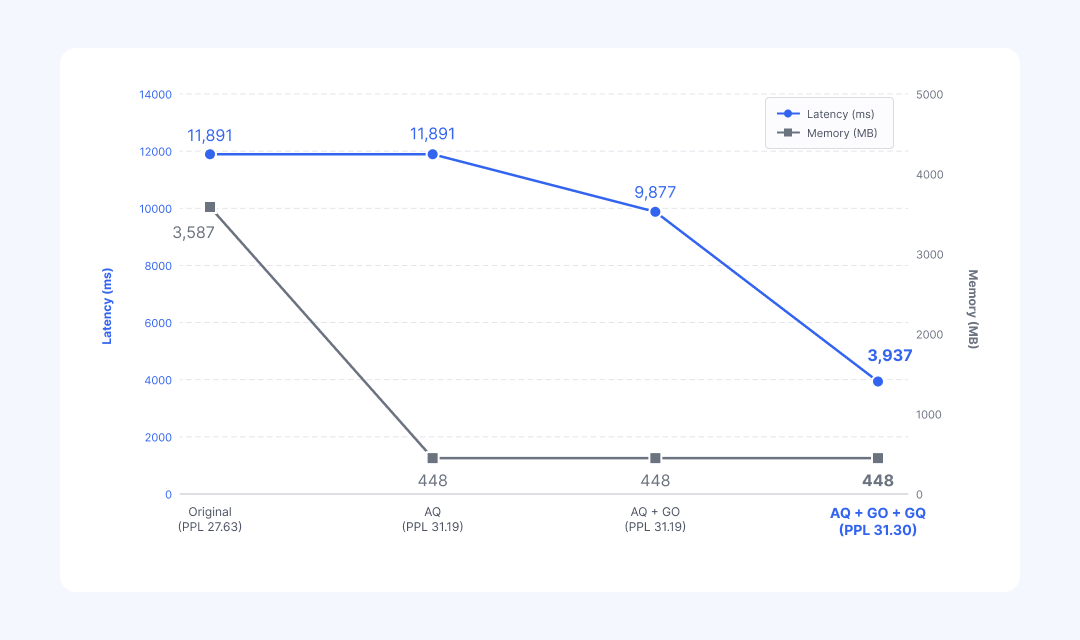
Table 6: Stage-by-stage changes in latency, memory, and PPL for the Llama 3.2 1B model across AQ → GO → GQ
Final Result: 67% Latency Reduction and 87% Memory Reduction (PPL 27.63 → 31.30). All of this is achieved with a single YAML configuration and one np run command.
This pipeline holds up just as well on very large models beyond 30B parameters. In a server-class LPU deployment project that Nota AI carried out, combining MXFP4, AWQ, and mixed precision techniques compressed the original model to roughly one-third of its size, while keeping accuracy loss within 1%.
💡 [The Same Pipeline Applies to NPU and Vision Models] While the previous example focused on a CPU environment, the pipeline applies equally to ultra-low-power NPUs (e.g., Arm Ethos-U). Even when the target is set to speech recognition (Conformer) or a vision model (ResNet50, etc.), the pipeline works without modification. When the target changes, the GO engine reassembles the graph accordingly. In fact, for vision models, passing through only GO and GQ without the AQ stage has delivered up to 42x speedups, demonstrating the pipeline's extensibility.
Without NetsPresso®: The Reality of a Six-Step Optimization Pipeline
Let us imagine building the AQ, GO, and GQ pipeline described so far without NetsPresso®. At a minimum, it would go through six fragmented stages, and each stage comes with its own trial and error.
PyTorch quantization: Environment conflicts across libraries such as autoawq, tokenizer setup for each model, and corpus preprocessing.
Graph conversion: Frequent failures of torch.onnx.export, and limited support for dynamic shapes and custom operators.
Graph optimization: Rules that require splitting on NPU and grouping on CPU have to be validated manually for each target.
Hardware quantization: TensorRT, OpenVINO, Vela, and other runtimes each demand entirely different toolchains and formats.
Cross-compilation: For embedded targets, setting up the cross-compile environment itself is a separate effort.
Profiling: Device warm-up, writing scripts for latency and memory measurement, and debugging back through measurement errors.
The biggest issue is that the input and output formats differ at every stage. Stitching these toolchains together takes significant effort. Moreover, if even one target device changes, steps 3 through 6 effectively have to be reconfigured from scratch.
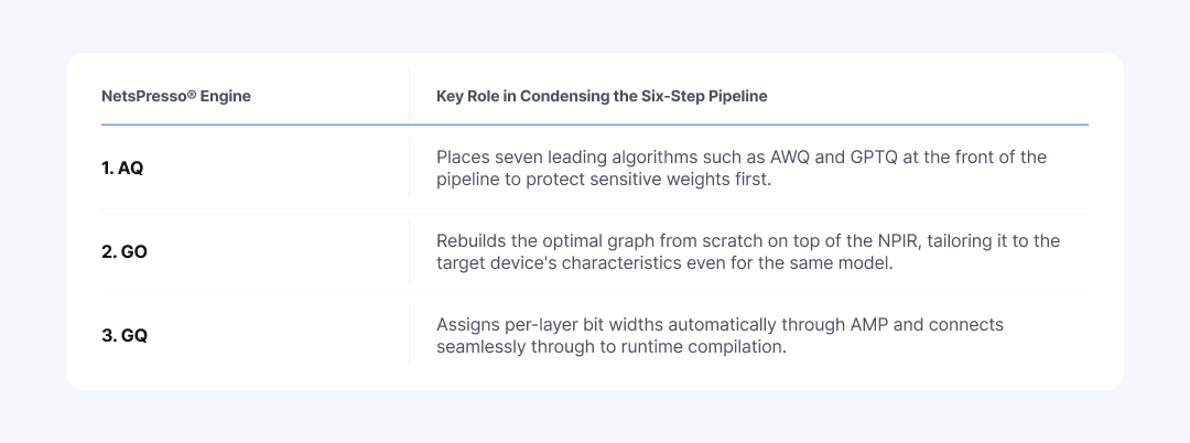
Table 7: Summary of how NetsPresso® AQ, GO, and GQ engines replace the six-step manual pipeline
Regardless of which model or device is chosen, the engineer has only one thing to do: write a single configuration file (YAML) and run the np run command once. With that alone, the entire optimization journey is completed automatically on top of NetsPresso®.
At the foundation of this pipeline lies the extensive hardware deployment experience that Nota AI has accumulated by working directly in the field over several years.
From the ultra-small Arm Cortex-M to NVIDIA Jetson, Intel Xeon, and AWS Inferentia, and up to recent NPUs such as Hailo-8 and FURIOSA RNGD, the real field data (pattern rules and quantization know-how) collected while deploying more than 100 AI models across diverse chipset environments forms the backbone of the NetsPresso® engines.
The AQ, GO, and GQ pipeline discussed in this post is available today through the NetsPresso® CLI. If you would like to try it with your own models, please explore it through the demo.
The benchmark numbers used in this post are results from a specific combination of model, hardware, and configuration, and actual performance may vary by environment.
If you have any further inquiries about this research, please feel free to reach out to us at following email address: 📧 contact@nota.ai.
Stay ahead with Nota AI on LinkedIn. From edge AI trends to the latest tech updates — subscribe to Edge Insights and be the first to know. 👉 Subscribe nowFurthermore, if you have an interest in AI optimization technologies, you can visit our website at 🔗 netspresso.ai.